Spectral Optimization for Neural Networks: Muon and the Newton-Schulz Iteration

Introduction

Optimization has been one of the central drivers of progress in modern machine learning. From early stochastic approximation methods to today’s large-scale neural network optimizers, the history of optimization in machine learning can be understood as a sequence of increasingly refined answers to the same question: how should we use noisy gradient information to make reliable progress towards a good solution?

Early stochastic gradient methods used random samples to estimate the direction of improvement [1], which helped make optimization scalable when computing the full gradient was expensive or intractable. In its simplest form, for a model $f$ with weight matrix $W$ trained on a dataset consisting of pairs ${(x_i,y_i)}_{i=1}^N$ and evaluated via a per-pair loss function $l(f(x_i),y_i)$, stochastic gradient descent (SGD) updates model parameters by

where $W_t$ denotes the weights at step $t$, $\eta$ is the learning rate, and $G_t$ is a stochastic estimate of the gradient:

where $L$ is the loss over the whole training dataset. In stochastic gradient descent, $G_t$ is computed over a randomly selected subset (referred to as a mini-batch, $B_t$) of the entire training dataset:

where $f_t$ denotes the model consisting of weights $W_t$ at step $t$.

Momentum methods, first introduced by Polyak in 1964 [2], accumulate a velocity term which helps to smooth noisy gradients and accelerate optimization along persistently helpful directions. A standard update of SGD with momentum (SGD-M) takes the form

where $M_t$ is an (un-normalized) moving average of past gradients and $\beta \in [0,1)$ controls how much past gradient information is retained. Later adaptive methods such as AdaGrad [3], RMSProp [4], and Adam [5] added per-coordinate learning rate adjustments. Adam, for instance, maintains both an exponential moving average of past gradients (the first moment) $m_t$ as well as squared gradients (the second moment) $v_t$:

where $m$, $v$, and $g$ refer to a given weight in the weight matrix. After normalizing by the long-run sum of weights $(1-\beta) \sum_{i=1}^t \beta^{t-i} = 1-\beta^t$ to account for the smallness of $m$ and $v$ for the first few steps (since gradient descent begins with no momentum),

the weight update is given by

where all operations are performed entry-wise.

This combination of momentum and per-coordinate rescaling helped establish Adam as the default optimizer for many deep learning systems.

A separate but equally relevant line of research centers around Newton-Schulz iteration. In 1933, Schulz produced his seminal work on iterative matrix inversion [6], which later became part of a broader family of matrix polynomial methods for computing inverses, inverse square roots, and in particular, polar factors.

The polar factor of a matrix appears through the singular value decomposition (SVD). For a real matrix $X$ with SVD $U \Sigma V^T$, the polar factor of $X$ is $UV^T$. Computing the polar factor effectively removes the singular value scaling $\Sigma$ while preserving the left and right singular directions, thereby producing an orthogonal matrix — in particular, this orthogonalization process produces the nearest orthogonal matrix to $X$ as measured by the Frobenius norm, as noted by Higham’s influential paper in 1986 [7]:

A few years earlier in 1971, Björck and Bowie [8] were the first to explicitly provide a family of polynomial iterative algorithms for computing the nearest orthogonal matrix based on the identity

which applies when $X$ is full column rank. In particular, for $Q = I - X^T X$,

and truncating to different orders produces various classic polynomials used for Newton-Schulz iteration updates, such as the commonly used quintic Newton-Schulz form,

The 2024 Muon optimizer connects these two histories, linking neural network optimization to classical matrix orthogonalization [9]. Instead of re-scaling coordinate-wise as Adam does, Muon instead iteratively orthogonalizes the momentum matrix, re-scaling the singular values towards (approximately) 1, making the inductive bias that a balanced set of singular directions leads to likely better quality weight updates than a balanced set of weight entries.

Today, SGD, SGD-M (SGD with momentum), Adam, and Muon are all used in practice, with Adam and Muon being the two optimizers used for the vast majority of modern large-scale model training. Further refinements to Muon have also been developed recently, such as Gram-Newton-Schulz, which makes use of the momentum’s Gram matrix, $MM^T$, to reduce the number of expensive rectangular matrix multiplications required.

Limitations of Adam

A major limitation of Adam, and one of the main reasons for the development of Muon [9], was its propensity to produce weight updates with large condition numbers.

Consider, as a toy example, the weight matrix $W \in \mathbb{R}^{2 \times 1}$. Absorbing the small $\varepsilon$ term in Adam’s weight update step (present to prevent division by zero) into $\hat{v}_w$, dropping the hat symbol for notational convenience, and rewriting the update step in matrix form,

Suppose the gradients are given by

and on each gradient update step,

with $\varepsilon_i \sim N(0,1)$ on each gradient update step.

Then since $M$ and $V$ are exponential moving averages, they converge over the gradient update steps towards $\mu$ and $\mu^2 + \sigma^2$ respectively. Thus, if, say, due to labels with differing levels of noise, $\sigma_2 \gg \sigma_1$,

can have a much smaller lower entry than upper entry, implying a greatly amplified condition number. For instance, with $\mu_1 = 1, \sigma_1 = 1, \mu_2 = 0.1, \sigma_2 = 100$, the condition number of the “true gradient matrix”

is amplified by about 70 times to give $M/\sqrt{V}$, in turn giving $\Delta W$ a large condition number.

Since the condition number is given by $\kappa(\Delta W) = \sigma_{max}/\sigma_{min}$, where $\sigma_{max}$ and $\sigma_{min}$ are the maximum and minimum singular values of $\Delta W$ respectively, this implies a dangerous tradeoff. If the condition number is large, then $\sigma_{max}$ and $\sigma_{min}$ are far apart, so we need to choose $\eta$ such that the largest direction in parameter space (corresponding to $\sigma_{max}$) doesn’t diverge. However, this forces weight updates in the smallest singular direction to be very small, limiting the rate of convergence.

This example and the issue of $\Delta W$’s ill-conditioning hints at a fundamental problem with Adam’s “per-coordinate” rather than “matrix-based” approach: it struggles to recognize the relationships between weights and features which must learn together, as exemplified by the singular directions.

Muon

Muon, or Momentum Orthogonalized by Newton-Schulz, was proposed as an optimizer for 2D linear layers in neural networks [9]. Like SGD-M, Muon first forms a momentum matrix, but unlike Adam, it does not divide coordinate-wise by the moving average of the squared gradient. Instead, Muon orthogonalizes the momentum matrix before using it as the update direction.

Newton-Schulz iteration

The central computational problem in Muon is the orthogonalization step

Why not compute the SVD explicitly? Although the raw count of floating-point operations for certain SVD algorithms is comparable to iterative algorithms, the operations involved in a full SVD, such as Householder transformations, panel factorizations, and Givens rotations, are not as well matched to modern accelerator hardware as general matrix multiplications. Newton-Schulz iteration is attractive because it uses only matrix multiplications and linear combinations thereof.

Newton-Schulz iteration uses the key property that odd matrix polynomials act directly on the singular values. Suppose

Consider the polynomial iteration

If

then

and

Therefore

Equivalently, each singular value evolves independently according to the scalar polynomial

By choosing appropriate values of $a$, $b$, and $c$, it is thus possible to repeatedly apply the polynomial iteration to the momentum matrix $M$, pushing the singular values towards the desired fixed point of $1$ such that $M$ approximates the polar factor, $UV^T$.

Practical Muon implementations often use a quintic polynomial with coefficients $a=3.4445$, $b=-4.7750$, and $c=2.0315$. These values were chosen empirically by Muon author Keller Jordan [9], who observed that singular values in the range $[0.7, 1.3]$ were typically sufficient for good optimization performance, and using the above coefficients often enabled one to reach this range within only five iterations.

This convention can fail, however, for extremely ill-conditioned momentum matrices. If

is large, then after normalizing $M_t$ by $\lVert M_t\rVert_F$ to ensure that optimization does not diverge along the $\sigma_{max}$ singular direction, $\sigma_{max}\leq 1$ and $\sigma_{min}\ll 1$. For very small $\sigma$, the quintic update behaves approximately as

meaning the smallest singular values grow only by a factor of about $a$ per iteration. For extremely small singular values, many iterations may therefore be required before they approach the near-$1$ range.

Cost of Muon compared with SGD, SGD-M, and Adam

Let $W\in\mathbb{R}^{m\times n}$ with $m\leq n$, and let $P = mn$ denote the number of parameters in the matrix. Considering only the optimizer update and not the forward or backward pass, plain SGD has time complexity $O(P)$ and uses no additional memory.

SGD-M also has time complexity $O(P)$, but stores one additional momentum matrix, so its additional space cost is $O(P)$.

Adam’s first and second moment matrices take a constant number of operations per weight to compute, so it has time complexity $O(P)$. Storing these two additional matrices requires an additional space $O(P)$.

Muon has the same $O(P)$ memory scale, since it stores a momentum matrix and some temporary matrices during orthogonalization, but its optimizer step is more expensive. For Newton-Schulz applied to an $m\times n$ momentum matrix $M$, each iteration forms products such as

and then multiplies the resulting $m\times m$ matrix by $X_k$. The dominant rectangular multiplications cost $O(nm^2)$, while the square-shaped products cost $O(m^3)$. For $T$ Newton-Schulz iterations, the total optimizer cost is therefore $O(Tnm^2 + Tm^3)$. In large neural network training, this overhead is often tolerable because the forward and backward pass for a batch of size $B$ costs roughly $O(nmB)$, and in many large-batch training regimes $B\gg m$. The Newton-Schulz overhead is therefore comparatively negligible.

Gram-Newton-Schulz

Gram-Newton-Schulz is a recent refinement of the Newton-Schulz orthogonalization step designed to reduce the cost of Muon’s repeated rectangular matrix multiplications [10]. The baseline method improves the speed of Newton-Schulz, but at the cost of worse conditioning and the potential for greater numerical instability.¹

For $X=U\Sigma V^T$ with $X\in\mathbb{R}^{m\times n}$ and $m\leq n$, assuming full row rank,

Therefore

Thus one can compute the polar factor by forming the Gram matrix $R_0=XX^T$ and approximating $R_0^{-1/2}$. If $Q_T\approx R_0^{-1/2}$, then $Q_TX\approx UV^T$.

Thus, instead of standard Newton-Schulz where one repeatedly updates the large rectangular matrix $X_k$, Gram-Newton-Schulz performs the iterations on the smaller $m\times m$ matrix $R_k$.

To see the connection to ordinary Newton-Schulz, first consider the scalar case. Suppose a singular value $x$ is updated by the odd polynomial

Because the polynomial is odd, it can be factored as

where

Define $r_0=x_0^2$ and $q_0=1$, then set

and

The variable $r_t$ tracks the squared singular value after $t$ iterations, while $q_t$ accumulates the total multiplied scale factor applied to the original singular value. If Newton-Schulz succeeds in driving $x_T$ close to $1$, then

The matrix version lifts this scalar recurrence to the eigenvalues of $R_0=XX^T$. Analogous to the scalar variables above, $R_t$ tracks the squared singular values after the corresponding Newton-Schulz updates, $Z_t$ is the current scale factor, and $Q_t$ is the accumulated inverse-square-root-like correction. In exact arithmetic, this produces the same singular-value iteration as standard Newton-Schulz.

From Section 3.2, standard Newton-Schulz for $X\in\mathbb{R}^{m\times n}$ with $m\leq n$ has time complexity approximately $O(Tnm^2+Tm^3)$. The factor $Tnm^2$ appears because each iteration performs rectangular multiplications involving the full $m\times n$ matrix.

Gram-Newton-Schulz instead forms $R_0=XX^T$ once, costing $O(nm^2)$, then performs $T$ iterations on $m\times m$ matrices, costing $O(Tm^3)$, and finally multiplies $Q_TX$, which costs another $O(nm^2)$. The total cost is therefore $O(nm^2+Tm^3)$.

The main improvement is that the expensive rectangular multiplication is not performed $T$ times; the iteration is instead performed on the smaller Gram matrix.

Conditioning and stability of Gram-Newton-Schulz

Though Gram-Newton-Schulz provides a speed advantage, it comes at the cost of worse conditioning and instability. Forming the Gram matrix squares the condition number, since if $\kappa(X)=\sigma_{max}/\sigma_{min}$, then

Since Newton-Schulz first normalizes the singular values to lie within $[0,1]$, very small singular values become even smaller eigenvalues of the Gram matrix. Combined with the common use of low-precision floating point formats in machine learning, such as float16 or bfloat16, these tiny eigenvalues can be numerically unstable.

Mathematically, $XX^T$ is positive semidefinite, so its eigenvalues should be nonnegative. However, roundoff error can cause very small positive eigenvalues to become negative. Since the Gram recurrence updates eigenvalues according to

if $r_{t-1}<0$, then $r_t$ remains negative, and its magnitude can grow. In the worst case, this can cause the accumulated correction matrix $Q_t$ to diverge.

Implementation and experiments

Comparing Newton-Schulz and Gram-Newton-Schulz

To compare the behavior of Newton-Schulz and Gram-Newton-Schulz, I implemented both algorithms and tested them on matrices with prescribed singular values. One matrix was well-conditioned, with $\sigma_i\in[0.5,1]$, and another was ill-conditioned, with singular values $\sigma_i\in[10^{-14},1]$. The experiment used low-precision arithmetic (float16), to expose precision and roundoff effects. In particular, the ill-conditioned matrix is effectively numerically singular given that its condition number is well below the machine precision of float16.

The first comparison measured the convergence of the singular values toward $1$ as a function of estimated cumulative floating-point operations. FLOPs were estimated manually using the approximation that multiplying an $a\times b$ matrix by a $b\times c$ matrix costs approximately $2abc$ floating point operations.

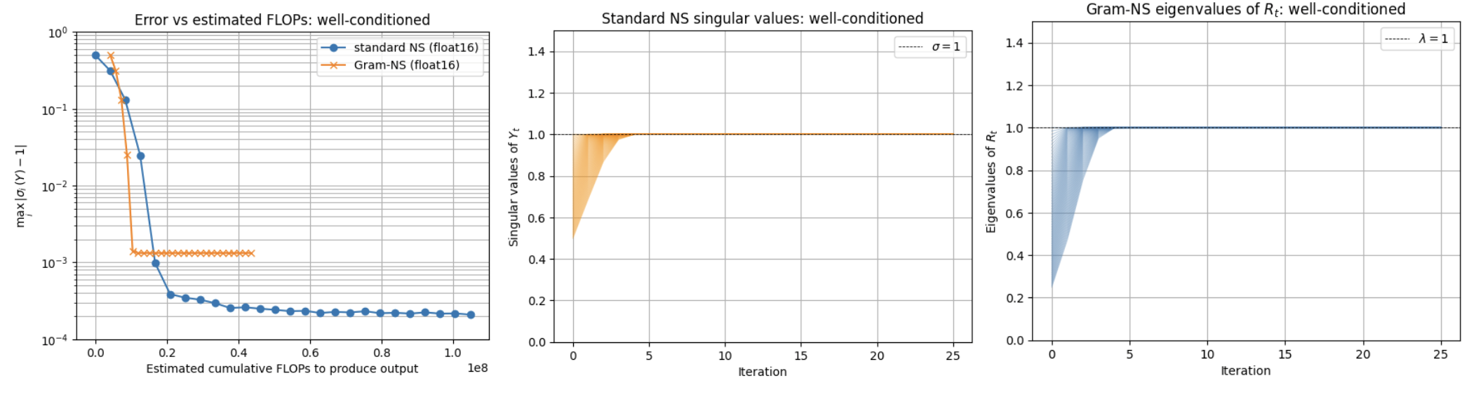
For the well-conditioned matrix (see Fig. 1), both methods rapidly move the singular values toward $1$. Standard Newton-Schulz reached a lower precision floor, likely because the standard iteration directly updates the output matrix $Y_k$, and the fixed point at singular value $1$ is super-attractive, meaning that if roundoff pushes a singular value slightly away from $1$, the next iteration tends to pull it back. For Gram-Newton-Schulz, roundoff errors in $Q_k$ are not “automatically” mitigated in this way, resulting in a higher, flatter precision floor.

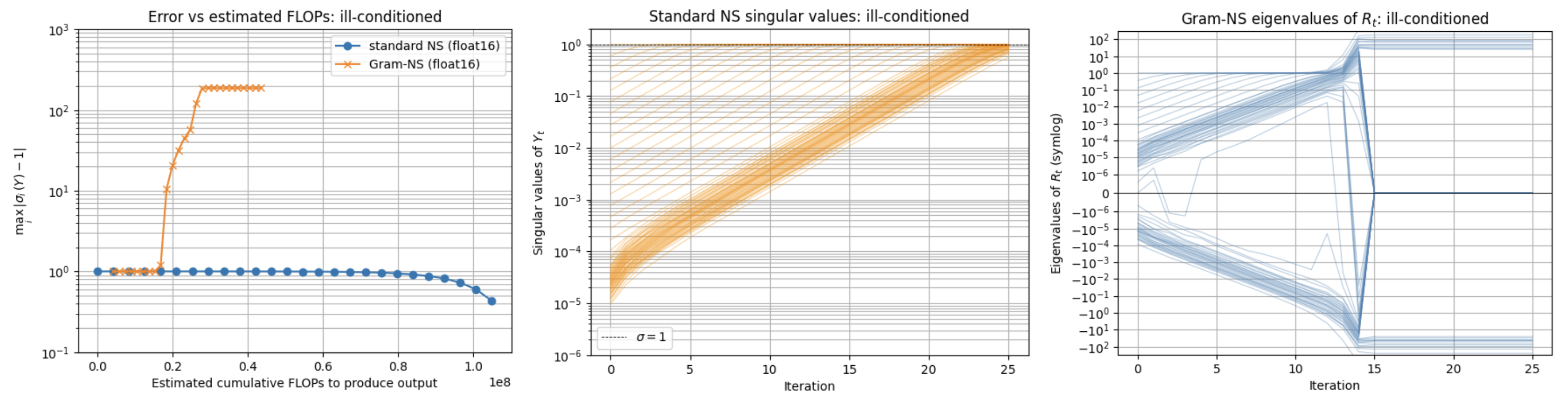
For the ill-conditioned matrix (see Fig. 2), standard Newton-Schulz remained stable but required many more iterations to scale up the smallest singular values. This is expected, since $p(\sigma)\approx a\sigma$ when $\sigma\ll 1$, and therefore more multiplicative iterations are required for the smallest singular values to approach 1.

Gram-Newton-Schulz was unstable in the ill-conditioned case, and singular values deviated significantly from 1 according to the left-side plot. From the right-side plot, it appears that roundoff error caused some negative eigenvalues to appear in the Gram matrix $R=XX^T$, which were then amplified by the recurrence $r_t=r_{t-1}h(r_{t-1})^2$, leading to divergence (before being clipped at around $\pm 10^2$).

Optimizer comparison experiment

I also compared SGD, SGD-M, Adam, and Muon on a controlled teacher-student regression task. The model consisted of a single $32\times 32$ linear layer. A fixed teacher matrix $W^{\ast}$ generated clean labels

while the student model predicted

The training dataset consisted of input-output pairs with noisy labels $(x_i, y_i+\varepsilon_i)$, so the training loss for a batch of size $B$ was

The test loss was evaluated on unseen pairs $(x_i, y_i)$:

Each experiment was run over multiple random seeds and averaged.

No-noise setting

In the no-noise setting (see Fig. 3), Muon exhibited a nearly fixed Frobenius norm weight update.

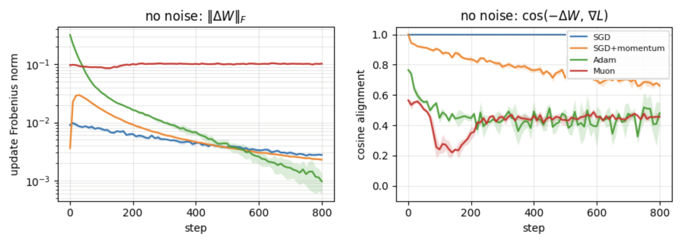
This occurs because the orthogonalized update has singular values near $1$, so for a $32\times 32$ square matrix, $\lVert\Delta W\rVert_F \approx \eta\sqrt{32}$. With $\eta=0.02$, this is approximately $0.02\sqrt{32}\approx 0.11$.

By contrast, SGD, SGD-M, and Adam showed shrinking update norms as the gradient magnitude decreased over training.

Cosine alignment between the weight update and the negative gradient also differed across optimizers. SGD is, by definition, maximally aligned with the current negative gradient. Adam is less aligned because coordinate-wise rescaling changes the direction of the update. Muon is also less aligned because orthogonalization redistributes the update across singular directions. This is not necessarily a weakness: Muon deliberately chooses a direction that is more spectrally balanced rather than one that exactly follows the raw gradient — this plot serves rather as validation that Muon behaves as expected relative to other optimizers.

Failure mode: noisy but important coordinates

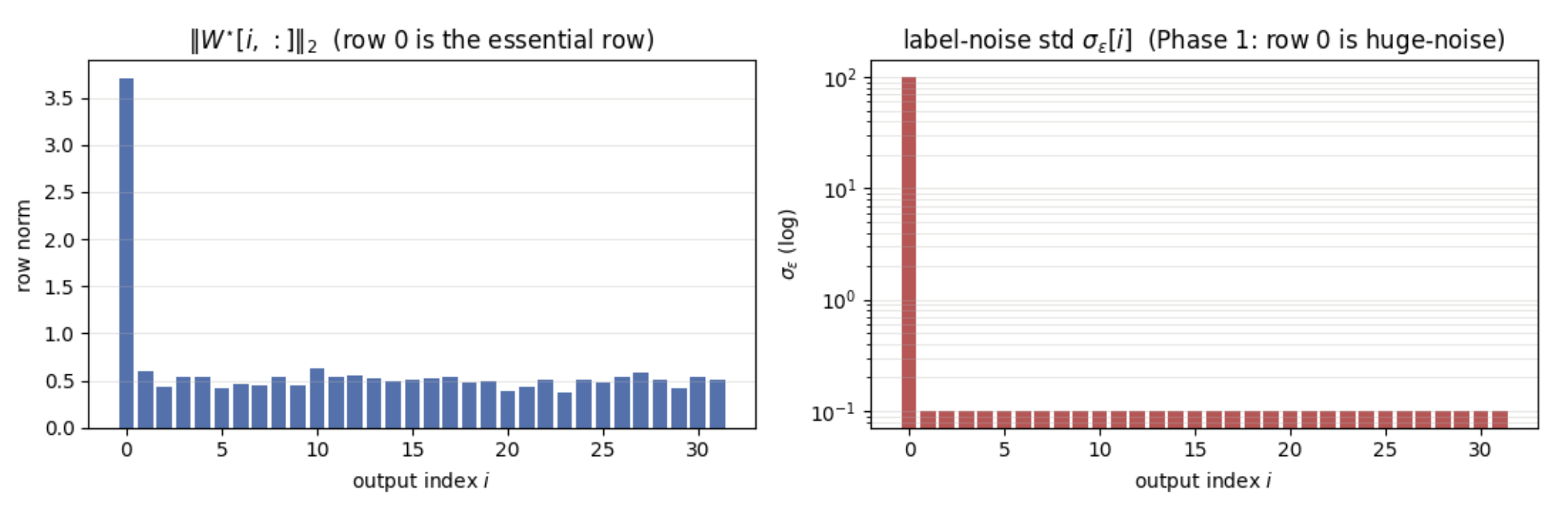
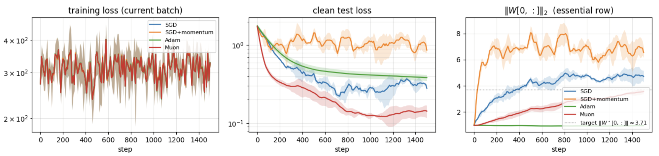
The first noisy experiment was designed to expose a failure mode of Adam in over-suppressing a noisy but important signal. The target matrix $W^{\ast}$ was constructed so that row $0$ contained the most important learning signal. However, row $0$ also had much larger label noise than the other rows (see Fig. 4). Thus the optimizer faced a tension: it needed to keep learning an important row despite the fact that gradients in that row were highly noisy.

In this experiment (see Fig. 5), the current-batch training loss was extremely noisy because it was dominated by irreducible label noise. From the test loss plot, SGD learned the important row but overshot its target norm due to random walk effects induced by the noisy gradients. SGD-M overshot even more likely because momentum amplified persistent noise. Adam, by contrast, strongly suppressed the noisy row: its second-moment estimate was large in that coordinate, so the effective learning rate became small. As a result, Adam under-learned the row that mattered most. Muon performed best in this setting. By orthogonalizing the momentum matrix, Muon avoided suppressing the important noisy row as aggressively as Adam, while also avoiding the large random-walk overshoot of SGD and SGD with momentum. In the experiment, the target row norm was approximately $|W^{\ast}_{0,:}|_2\approx 3.71$, and Muon landed closest to this value.

Failure mode: phase switch

The second noisy experiment (see Fig. 6) introduced a “phase switch”. Before step $500$, row $0$ was very noisy. After step $500$, the noise in row $0$ dropped sharply. This experiment tested whether optimizers could recover once a previously noisy but important coordinate became clean.

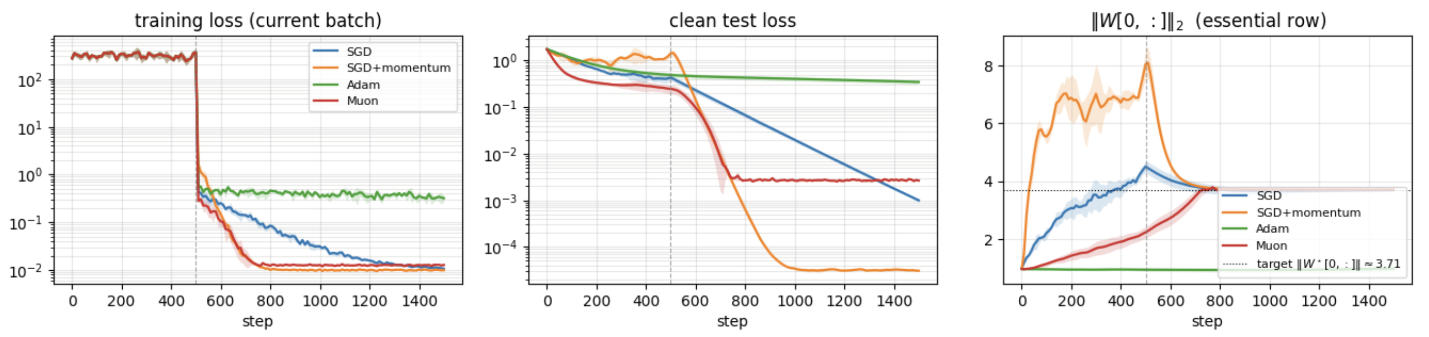
After the noise dropped, SGD recovered, and SGD with momentum recovered even faster. Muon also recovered, though in the clean-gradient phase SGD and SGD with momentum eventually outperformed it — once the gradients became clean and well-aligned, the raw gradient direction was highly informative, and the additional spectral balancing imposed by Muon was less helpful.

Notably, Adam recovered poorly. Its second-moment estimate retained memory of the earlier high-noise phase, and therefore Adam continued to use a small effective learning rate for row $0$ even after that row became clean. This demonstrates a common failure mode of Adam’s coordinate-wise adaptivity: it can suppress important directions based on past noise, even after the noise distribution changes.

Condition number behavior

The condition number $\kappa(\Delta W)$ of the update matrix was also visualized for sake of validation (see Fig. 7).

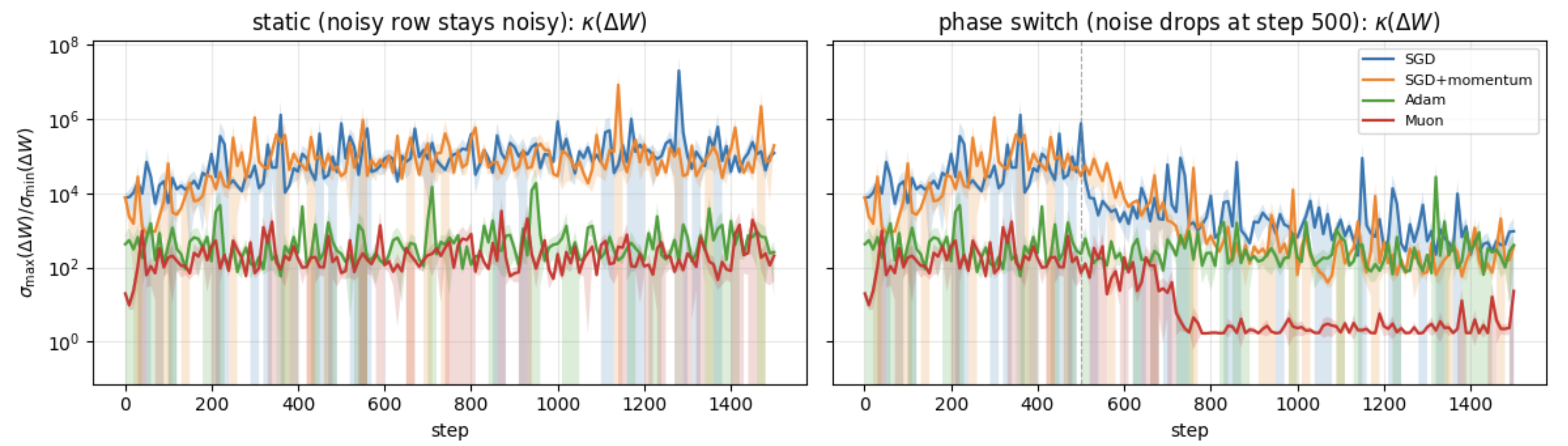
As expected, Muon maintained comparatively low condition number because its update is constructed to have singular values near $1$. SGD and SGD with momentum inherited the anisotropy and noise structure of the problem, producing much larger condition numbers. In the static noisy-row setting, the momentum matrix contained stochastic noise throughout training, so even $T=5$ Newton-Schulz iterations were not always sufficient to bring Muon’s condition number near $1$. In the phase-switch setting, once the noise dropped away, Muon’s condition number quickly returned close to $1$.

Adam vs Muon: when to use which

Muon and Adam encode fundamentally different inductive biases. Adam assumes that the right unit of adaptation is the individual weight coordinate: each parameter receives its own effective learning rate based on the history of its gradient magnitude. Muon assumes that, for linear 2D hidden matrices, the right unit of adaptation is the singular direction: the optimizer should balance singular directions rather than matrix entries.

There is no general theorem saying that balancing singular directions is always better than balancing coordinates — Muon’s advantage depends on the structure of the problem. In practice, Muon has been found to be most appropriate when the parameter has meaningful matrix structure, as in large dense linear 2D layers. In such layers, rows and columns represent interacting learned features, and the SVD can capture coordinated directions of change.

Adam remains a safe default in many settings, especially for parameters where coordinates are naturally separate or sparse. In the input and output layers of language models, for instance, different rows correspond to different vocabulary items, and it does not make as much sense to consider mixing between coordinate entries via the singular directions. Rather, the sparse token frequencies make coordinate-wise adaptivity useful. In addition, for non-linear and non-2D layers, Adam is also usually preferred, since the matrix-specific benefits of Muon no longer tend to apply.

A practical modern recipe therefore takes a hybrid approach: use Muon for 2D hidden weight matrices where important learning directions may well span across weight coordinates, and use Adam for input/output layers, nonlinear layers, and other non-matrix structures. This hybrid approach preserves Adam’s robustness where coordinate-wise adaptivity is useful, while exploiting Muon’s matrix-aware spectral balancing where the parameter structure supports it.

References

1. H. Robbins and S. Monro, "A Stochastic Approximation Method," The Annals of Mathematical Statistics, 22(3):400–407, 1951. doi:10.1214/aoms/1177729586
2. B. T. Polyak, "Some methods of speeding up the convergence of iteration methods," USSR Computational Mathematics and Mathematical Physics, 4(5):1–17, 1964. doi:10.1016/0041-5553(64)90137-5
3. J. Duchi, E. Hazan, and Y. Singer, "Adaptive subgradient methods for online learning and stochastic optimization," Journal of Machine Learning Research, 12(7), 2011.
4. T. Tieleman and G. Hinton, "Lecture 6.5—RMSProp: Divide the gradient by a running average of its recent magnitude," Coursera: Neural Networks for Machine Learning, 4(2):26, 2012.
5. D. P. Kingma and J. Ba, "Adam: A Method for Stochastic Optimization," arXiv preprint arXiv:1412.6980, 2014. arxiv.org/abs/1412.6980
6. G. Schulz, "Iterative Berechnung der reziproken Matrix," ZAMM — Journal of Applied Mathematics and Mechanics, 13(1):57–59, 1933.
7. N. J. Higham, "Computing the polar decomposition—with applications," SIAM Journal on Scientific and Statistical Computing, 7(4):1160–1174, 1986.
8. Å. Björck and C. Bowie, "An iterative algorithm for computing the best estimate of an orthogonal matrix," SIAM Journal on Numerical Analysis, 8(2):358–364, 1971.
9. K. Jordan, Y. Jin, V. Boza, J. You, F. Cesista, L. Newhouse, and J. Bernstein, "Muon: An Optimizer for Hidden Layers in Neural Networks," Keller Jordan Blog, 2024. kellerjordan.github.io/posts/muon
10. T. Dao, J. Zhang, N. Amsel, and B. Chen, "Gram Newton-Schulz: A Fast, Hardware-Aware Newton-Schulz Algorithm for Muon," Tri Dao Blog, 2026. tridao.me/blog/2026/gram-newton-schulz